Module 24: Data Science

Learning Objectives

• Understand the role of Python in data science.
• Set up a Python environment for data science tasks.
• Import, clean, and manipulate datasets using Python libraries.
• Perform exploratory data analysis using Python.
• Create visualizations to analyze and interpret data.

 

1. Introduction to Data Science

Data science is a highly relevant interdisciplinary field that integrates statistical methods, computer science, and domain-specific expertise to uncover actionable insights and generate knowledge from both structured and unstructured data. It encompasses a wide range of processes, including data acquisition, cleaning, exploration, analysis, modeling, and visualization, all aimed at facilitating data-driven decision-making. Data science leverages advanced techniques such as machine learning, predictive analytics, and big data technologies and empowers organizations to address complex challenges, identify patterns, and forecast future trends. Its applications span diverse industries, including healthcare, where it aids in disease prediction and personalized treatment; finance, where it enhances risk management and fraud detection; marketing, where it drives customer segmentation and targeted campaigns; and technology, where it fuels artificial intelligence and automation.

Here are a few examples of data science applications.

• Data science is used by the healthcare industry and organizations to make instruments to detect and cure disease.
• It is used in identifying patterns in images and finding objects in images.
• It is used to show the best results for our searched query, a search engine uses data science algorithms.
• Data science algorithms are used in digital marketing which includes banners on various websites, billboards, posts etc. those marketing are done by data science. Data science helps to find the correct user to show a particular banner or advertisement.
• Logistics companies ensure faster delivery of your order, so these companies use data science to find the best route to deliver the order.

 

2. Python for Data Science

Python is a leading programming language in data science, celebrated for its simplicity, flexibility, and rich ecosystem of libraries and tools. Its user-friendly syntax and readability make it accessible to both beginners and experts, while its versatility supports a wide range of data science applications. Core libraries like pandas and NumPy deliver robust solutions for data manipulation and numerical analysis, enabling users to handle complex datasets with ease. Visualization tools such as Matplotlib and Seaborn empower data scientists to create insightful and aesthetically appealing graphs and charts. For machine learning, Python provides cutting-edge frameworks like scikit-learn, TensorFlow, and PyTorch, offering comprehensive capabilities for building and deploying predictive models. Python’s seamless integration with other software tools and platforms, coupled with its vast and supportive community, enhances its efficiency for managing the entire data science workflow—from data preprocessing to advanced modeling and deployment. Its adaptability and ecosystem make it an indispensable asset for modern data science projects.

 

3. Introduction to NumPy and Its Importance in Data Science

NumPy stands for Numerical Python, is an open-source Python library that provides support for large, multi-dimensional arrays and matrices. It provides tools for numerical computations and forms the foundation of many other data science libraries like pandas, scikit-learn, and TensorFlow, making it essential for anyone working in data science. NumPy offers robust functionality for handling and manipulating multi-dimensional arrays, performing mathematical operations, and enabling efficient data processing.

The library is particularly useful for:

• Handling large datasets: NumPy's arrays are optimized for efficient storage and computation, allowing it to handle large datasets effectively.
• Vectorized computations: It eliminates the need for loops by supporting operations on entire arrays at once.
• Integration with other libraries: Many Python data science libraries use NumPy arrays as their base data structure.

Key Features of NumPy

NumPy offers a range of features that make it a preferred choice over Python lists for numerical computations. Some of its most notable features include:

• Powerful N-dimensional array object: Enables efficient storage and manipulation of multi-dimensional data.
• Sophisticated broadcasting functions: Simplifies mathematical operations on arrays of different shapes.
• Integration with C/C++ and Fortran: Provides tools for seamless interaction with low-level code for enhanced performance.
• Advanced mathematical capabilities: Includes functions for linear algebra, Fourier transforms, and random number generation.

In addition to its scientific applications, NumPy serves as an efficient multi-dimensional container for generic data. It supports the definition of arbitrary data types, allowing it to integrate seamlessly and efficiently with diverse databases.

Install Python NumPy

Numpy can be installed for Mac and Linux users via the following pip command:

pip install numpy

Windows does not have any package manager analogous to that in Linux or Mac. You can download the pre-built Windows installer for NumPy.

Once NumPy is installed, import it in your applications by adding the import keyword:

import numpy

Now NumPy is imported and ready to use.

import numpy arr = numpy.array([1, 2, 3, 4, 5,6,7,8,9,10]) print(arr)

Output:

[ 1 2 3 4 5 6 7 8 9 10 ]

Arrays in NumPy

The core structure in NumPy is the homogeneous multidimensional array, which forms the foundation of its functionality.

• Definition: A NumPy array is a table of elements (typically numbers) where all elements are of the same data type. Each element is accessed using a tuple of positive integers as indices.
• Axes and Rank: In NumPy, the dimensions of an array are referred to as axes, and the total number of axes is called the rank.
• Array Class: NumPy arrays are represented by the ndarray class, often referred to simply by its alias, array.

Example:

In this example, a two-dimensional array is created that has the rank of 2 as it has 2 axes.

The first axis(dimension) is of length 2, i.e., the number of rows, and the second axis(dimension) is of length 3, i.e., the number of columns. The overall shape of the array can be represented as (2, 3)

Output:

NumPy Array Creation

There are various ways of Numpy array creation in Python. They are as follows:

1. Create NumPy Array with List and Tuple

You can create an array from a regular Python list or tuple using the array() function. The type of the resulting array is deduced from the type of the elements in the sequences.

import numpy as np # Creating array from list with type float a = np.array([[1, 2, 4], [5, 8, 7]], dtype = 'float') print ("Array created using passed list:\n", a) # Creating array from tuple b = np.array((1 , 3, 2)) print ("\nArray created using passed tuple:\n", b)

Output:

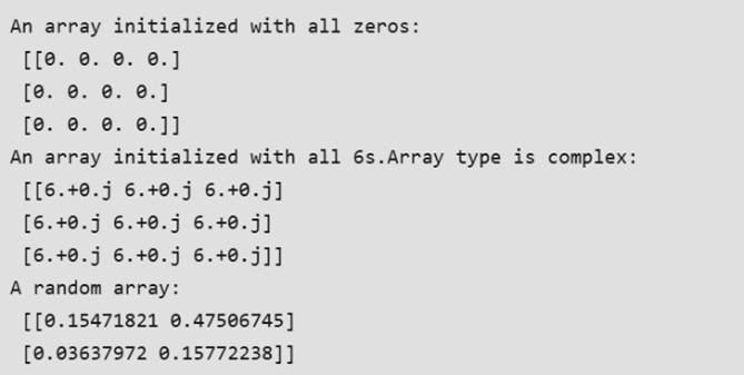
In many scenarios, the elements of an array are initially unknown, but the size is predetermined. NumPy provides several functions to create arrays with placeholder content, which helps avoid the computational expense of dynamically growing arrays.

Examples of such functions include:

• np.zeros: Creates an array filled with zeros.
• np.ones: Creates an array filled with ones.
• np.full: Creates an array filled with a specified value.
• np.empty: Creates an array without initializing its values (use with caution).

2. Creating Sequences

For generating sequences of numbers, NumPy offers functions similar to Python's range, but these return arrays instead of lists. These functions are highly efficient and versatile for numerical computations.

Output:

3. Create Using arange() Function

This function arange() function returns evenly spaced values within a given interval. Step size is specified.

# Create a sequence of integers # from 0 to 30 with steps of 5 f = np.arange(0, 30, 5) print ("A sequential array with steps of 5:\n", f)

Output

4. Create Using linspace() Function

linspace(): It returns evenly spaced values within a given interval.

# Create a sequence of 10 values in range 0 to 5 g = np.linspace(0, 5, 10) print ("A sequential array with 10 values between"                                  "0 and 5:\n", g)

Output:

5. Reshaping an Array Using the reshape Method

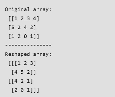
The reshape method allows us to modify the shape of an array while maintaining its original size.

For example, consider an array with the shape (a1,a2,a3,…,aN)(a_1, a_2, a_3, \dots, a_N)(a1​,a2​,a3​,…,aN​). This array can be reshaped into another array with the shape (b1,b2,b3,…,bM)(b_1, b_2, b_3, \dots, b_M)(b1​,b2​,b3​,…,bM​), provided the condition a1×a2×a3×⋯×aN=b1×b2×b3×⋯×bMa_1 \times a_2 \times a_3 \times \dots \times a_N = b_1 \times b_2 \times b_3 \times \dots \times b_Ma1​×a2​×a3​×⋯×aN​=b1​×b2​×b3​×⋯×bM​ is satisfied. In other words, the total number of elements in the array must remain the same after reshaping.

Output:

NumPy Array Indexing

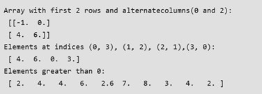
Understanding the fundamentals of NumPy array indexing is crucial for efficiently analyzing and manipulating array objects. NumPy provides several methods for array indexing:

• Slicing: Similar to Python lists, NumPy arrays support slicing. Since arrays can be multidimensional, a slice must be defined for each dimension of the array.

• Integer Array Indexing: This method uses lists of indices to select elements for each dimension. A one-to-one mapping is performed, allowing the creation of a new arbitrary array from the selected elements.
• Boolean Array Indexing: This technique is useful for selecting elements that meet specific conditions. A Boolean mask is applied to the array, returning only the elements that satisfy the given criteria.

Output:

4. Pandas DataFrame

The Pandas DataFrame is a versatile, two-dimensional, size-mutable, and potentially heterogeneous data structure that organizes data in a tabular format with labeled axes—rows and columns. It is a core component of the Pandas library and widely used for data manipulation and analysis in Python.

A DataFrame represents data in a spreadsheet-like format, where rows and columns align seamlessly. This structure makes it intuitive for handling and analyzing datasets of varying complexity and size. The three primary components of a Pandas DataFrame are:

• Data: The core content, which can include values of different types (e.g., numeric, categorical, string, or even complex objects).
• Rows: Represent observations or entries in the dataset, each uniquely identified by an index.
• Columns: Represent features, variables, or attributes, each labeled with a unique name for easy identification.

Pandas DataFrames are highly flexible and support various operations such as filtering, grouping, merging, reshaping, and applying functions, making them indispensable for data analysis and preprocessing tasks. Their capability to handle diverse data types, combined with powerful built-in methods, makes DataFrames a cornerstone of data science workflow.

Installing Pandas

Installing Pandas is straightforward if Python and PIP are already set up on your system.

You can install Pandas by running the following command in your terminal or command prompt:

bash pip install pandas

If the installation fails, consider using a Python distribution that includes Pandas by default, such as Anaconda or Spyder. These distributions provide an all-in-one environment for data analysis and scientific computing.

Importing Pandas

After installing Pandas, you can import it into your Python application using the import keyword:

python import pandas

Once imported, Pandas is ready for use. Here's an example demonstrating its functionality:

Example

This code creates a Pandas DataFrame from a dictionary and prints its content.

Importing Pandas as pd

In Python, Pandas is typically imported using the alias pd for convenience and readability.

What is an Alias?

An alias is an alternative name that can be used to refer to the same object. When importing a library, you can assign an alias using the as keyword.

Creating an Alias for Pandas

Use the following syntax to import Pandas with the pd alias:

import pandas as pd

With this alias, you can refer to the Pandas library as pd instead of typing the full name.

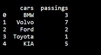
Example

This example demonstrates creating and printing a Pandas DataFrame using the pd alias.

Pandas Series

What is a Series?

A Pandas Series is similar to a column in a table. It is a one-dimensional array capable of holding data of any type.

Example: Creating a Series

Here’s how to create a simple Pandas Series from a list:

import pandas as pd a = [1, 7, 2] myvar = pd.Series(a) print(myvar)

Output:

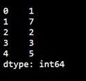
Labels

By default, the values in a Pandas Series are labeled using their index numbers. The first value has an index of 0, the second value has an index of 1, and so on. These labels can be used to access specific values.

Example: Accessing a Value by Index

# Return the first value of the Series print(myvar[0])

Output:

1

Creating Custom Labels

You can define your own labels for a Series using the index argument.

Example: Custom Labels

import pandas as pd a = [1, 7, 2] # Create a Series with custom labels myvar = pd.Series(a, index=["x", "y", "z"]) print(myvar)

Output:

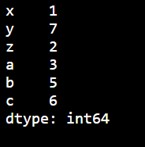
Accessing Values Using Custom Labels

Once custom labels are defined, you can access values by referring to these labels.

Example: Accessing a Value by Label

import pandas as pd a = [1, 7, 2] myvar = pd.Series(a, index = ["x", "y", "z"]) print(myvar["y"])

Output:

7

Creating a Pandas DataFrame

A Pandas DataFrame can be created by loading datasets from various storage sources, including SQL databases, CSV files, Excel files, and even JSON files. Additionally, DataFrames can be constructed directly from Python data structures such as lists, dictionaries, or even lists of dictionaries. This flexibility allows data to be easily imported from external sources or created programmatically within Python, enabling seamless data manipulation and analysis. The DataFrame is a powerful data structure in Pandas, ideal for handling and transforming data for a wide range of applications, from simple analyses to complex data processing workflows.

Here are some ways by which we create a dataframe:

Creating a dataframe using List: DataFrame can be created using a single list or a list of lists.

import pandas as pd   # list of strings list = ['Python', 'for', 'Data', 'Science']   # Calling DataFrame constructor on list df = pd.DataFrame(list) print(df)

Output:

Creating DataFrame from dict of ndarray/lists: To create DataFrame from dict of narray/list, all the narray must be of same length. If index is passed then the length index should be equal to the length of arrays. If no index is passed, then by default, index will be range(n) where n is the array length.

# Python code demonstrate creating # DataFrame from dict narray / lists # By default addresses.   import pandas as pd   # initialize data of lists. data = {'Name':['Kim', 'Seol', 'Park', 'Cho'],         'Age':[20, 21, 19, 18]}   # Create DataFrame df = pd.DataFrame(data)   # Print the output. print(df)

Output:

Rows and Columns in Pandas DataFrame

A DataFrame is a two-dimensional data structure in Pandas, meaning that data is organized in rows and columns, like a table. This structure allows for efficient data manipulation and analysis. In Pandas, we can perform a variety of operations on rows and columns, including selecting, deleting, adding, and renaming.

• Selecting: Rows or columns can be selected using index labels or column names. For example, you can use df['column_name'] to select a column or df.iloc[] for row-based indexing.
• Deleting: Rows or columns can be deleted using the drop() method. You can remove specific rows or columns by specifying their index or column name, and you can choose to modify the DataFrame in place or return a new one.
• Adding: New rows or columns can be added to the DataFrame by directly assigning values. For example, df['new_column'] = values will add a new column, while df.loc[index] = row_values can be used to append a new row.
• Renaming: Columns and rows can be renamed using the rename() method, where you provide a dictionary mapping old names to new ones.

Column Selection:
To select a column in a Pandas DataFrame, we can access it by its column name. This is done by using the column name within square brackets, like df['column_name']. This allows you to extract the column as a Pandas Series, making it easy to perform further operations on it. You can also select multiple columns by passing a list of column names, such as df[['col1', 'col2']].

Row Selection:
Pandas provides several methods to retrieve rows from a DataFrame.

• The loc[] method is used for label-based row selection. It allows you to select rows by their index labels, such as df.loc[2] to retrieve the row with index 2, or df.loc[2:5] to select a range of rows from index 2 to 5.
• The iloc[] method, on the other hand, is used for integer-location based indexing. This allows you to select rows by their integer position in the DataFrame, such as df.iloc[2] to select the third row (remembering that indexing starts at 0).

# Import pandas package import pandas as pd   # Define a dictionary containing employee data data = {'Name':['Mike', 'Bob', 'Kate', 'Josh'],         'Age':[27, 24, 22, 32],         'Address':['NY', 'GA', 'AZ', 'KY'],         'Qualification':['Msc', 'MA', 'MBA', 'Phd']}   # Convert the dictionary into DataFrame df = pd.DataFrame(data)   # select two columns print(df[['Name', 'Qualification']])

Output:

Working with Missing Data

Missing data arises when information is unavailable for certain entries in a dataset. This can occur at the item level (specific data points missing) or the unit level (entire rows or columns missing). Handling missing data effectively is crucial, as it can significantly impact the accuracy of analysis and modeling. In Pandas, missing data is typically represented as NaN (Not a Number) or NA (Not Available).

Checking for Missing Values

Pandas provides two essential functions to identify missing data:

• isnull(): This function returns a DataFrame or Series of the same shape, with True for missing (NaN) values and False otherwise.
• notnull(): This function does the opposite, returning True for non-missing values and False for missing ones.

These functions can be applied to both Pandas DataFrames and Series to locate missing values. For example:

import pandas as pd import numpy as np # Sample DataFrame with missing values data = {'Name': ['Alice', 'Bob', np.nan], 'Age': [25, np.nan, 30]} df = pd.DataFrame(data) # Check for missing values print(df.isnull()) # Check for non-missing values print(df.notnull())

Output:

Reading CSV Files with Pandas

CSV (Comma-Separated Values) files are a common format for storing large datasets in plain text, making them easily accessible and compatible with various tools, including Pandas.

Reading a CSV File into a DataFrame

You can load a CSV file into a Pandas DataFrame using the read_csv() method.

Example: Loading a CSV File

Here’s an example using a file named data.csv:

import pandas as pd # Load the CSV file into a DataFrame df = pd.read_csv('data.csv') # Display the entire DataFrame print(df.to_string())

The to_string() method is used to print the entire DataFrame, which can be especially useful for inspecting smaller datasets.

Notes:

• Ensure the CSV file is in the same directory as your script, or provide the full file path.
• Pandas automatically interprets the file format and reads the data efficiently.

 

5. Introduction to SciPy

What is SciPy?

SciPy is a robust library designed for scientific and technical computing, built on top of NumPy. It extends NumPy's functionality with advanced tools for tasks like optimization, integration, interpolation, eigenvalue problems, and signal and image processing.

• SciPy stands for Scientific Python.
• It is open-source, making it freely accessible and modifiable by the community.
• Created by Travis Oliphant, the same developer behind NumPy, SciPy has become a cornerstone of the Python scientific computing ecosystem.

Key Features of SciPy

SciPy offers a wide range of functionality, including:

• Optimization: Tools for minimizing or maximizing functions and solving systems of equations.
• Integration: Numerical integration of functions and solving ordinary differential equations (ODEs).
• Linear Algebra: Decomposition and matrix operations beyond what's available in NumPy.
• Statistics: Advanced statistical analysis tools, including probability distributions and hypothesis testing.
• Signal and Image Processing: Functions for filtering, Fourier transforms, and working with multi-dimensional image data.
• Sparse Matrices: Efficient storage and operations for matrices with a large number of zero entries.

Why Use SciPy?

Although SciPy is built on NumPy, it adds optimized and specialized functionality tailored to common scientific and data analysis workflows. Key benefits include:

• Efficiency: Functions in SciPy are often faster and better optimized than their NumPy equivalents.
• Breadth: SciPy provides tools for advanced tasks not covered by NumPy, reducing the need for additional libraries.
• Ease of Use: SciPy's APIs are designed to be intuitive, making complex mathematical operations accessible to users with basic Python knowledge.

Applications of SciPy

SciPy is widely used in fields such as:

• Physics, engineering, and mathematics for computational modeling.
• Data science and machine learning for statistical analysis and preprocessing.
• Signal and image processing for feature extraction and transformation.
• Economics and finance for optimization and integration tasks.

Language and Codebase

• Primary Language: SciPy is primarily written in Python for usability, with performance-critical components implemented in C for speed.
• Source Code: The complete SciPy codebase is hosted on GitHub, allowing developers to contribute or explore its implementation. You can find it here: SciPy GitHub Repository.

Why SciPy Matters

SciPy is more than just a library; it’s a tool that bridges the gap between theoretical computation and practical implementation. Its seamless integration with other Python libraries like NumPy, Matplotlib, and Pandas makes it a cornerstone of the Python scientific stack. Whether you're a researcher, engineer, or data scientist, SciPy empowers you to tackle complex computational problems with ease and precision.

Installing and Using SciPy

Installing SciPy

If Python and PIP are already installed on your system, installing SciPy is straightforward.

Use the following command to install SciPy:

pip install scipy

If the installation fails, consider using a Python distribution such as Anaconda or Spyder, which come with SciPy pre-installed and are ideal for scientific computing.

Importing SciPy 

Once SciPy is installed, you can import specific modules as needed using the from scipy import module syntax.

Example: Importing and Using the constants Module

The constants module in SciPy provides a wide range of mathematical and physical constants.

python from scipy import constants print(constants.liter)

In this example, the constants. Liter constant returns the equivalent of 1 liter in cubic meters. SciPy's constants module is a convenient resource for precise mathematical and physical values.

Checking the Installed SciPy Version

You can verify the installed version of SciPy using the __version__ attribute.

Example:

import scipy # Print the SciPy version print(scipy.__version_)

This command outputs the current version of SciPy, ensuring compatibility with your project or system requirements.

Constants in SciPy

As SciPy is more focused on scientific implementations, it provides many built-in scientific constants.

These constants can be helpful when you are working with Data Science.

from scipy import constants print(constants.pi)

Output:

3.141592653589793

Constant Units

A list of all units under the constants module can be seen using the dir() function.

from scipy import constants print(dir(constants))

Output:

Unit Categories

The units are placed under these categories:

• Metric
• Binary
• Mass
• Angle
• Time
• Length
• Pressure
• Volume
• Speed
• Temperature
• Energy
• Power
• Force

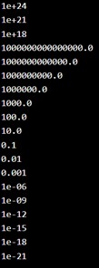
Metric (SI) Prefixes:

Return the specified unit in meter (e.g. centi returns 0.01)

from scipy import constants print(constants.yotta) print(constants.zetta) print(constants.exa) print(constants.peta) print(constants.tera) print(constants.giga) print(constants.mega) print(constants.kilo) print(constants.hecto) print(constants.deka) print(constants.deci) print(constants.centi) print(constants.milli) print(constants.micro) print(constants.nano) print(constants.pico) print(constants.femto) print(constants.atto) print(constants.zepto)

Output:

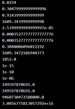
The final example is of length. Length: Return the specified unit in meters (e.g. nautical_mile returns 1852.0)

from scipy import constants print(constants.inch) print(constants.foot) print(constants.yard) print(constants.mile) print(constants.mil) print(constants.pt) print(constants.point) print(constants.survey_foot) print(constants.survey_mile) print(constants.nautical_mile) print(constants.fermi) print(constants.angstrom) print(constants.micron) print(constants.au) print(constants.astronomical_unit) print(constants.light_year) print(constants.parsec)

Output:

SciPy Optimizers

What are Optimizers in SciPy?

Optimizers in SciPy are a collection of tools designed to either:

• Minimize a function: Find the input values that result in the lowest output for a given function.
• Solve equations: Locate the roots of equations, where the function evaluates to zero.
• These tools are essential in scientific computing and machine learning, where optimization tasks and equation solving are fundamental.

Optimizing Functions

In machine learning and data analysis, algorithms often involve complex equations that need to be minimized or optimized based on the provided data. SciPy's optimization functions streamline this process.

Finding Roots of an Equation

While NumPy can handle roots for polynomials and linear equations, it lacks functionality for solving non-linear equations. SciPy addresses this limitation with the optimize.root function.

Using optimize.root

The optimize.root function locates the root of a non-linear equation. It requires:

• fun: A callable function representing the equation.
• x0: An initial guess for the root.

The function returns an object containing information about the solution. The actual root can be accessed using the .x attribute of the returned object.

Example

from scipy.optimize import root from math import cos def eqn(x):   return x + cos(x) myroot = root(eqn, 0) print(myroot.x)

Output:

[-0.73908513]

SciPy Sparse Data

What is Sparse Data

Sparse data is data that has mostly unused elements (elements that don't carry any information ).

It can be an array like this one:

[1, 0, 2, 0, 0, 3, 0, 0, 0, 0, 0, 0]

• Sparse Data: is a data set where most of the item values are zero.
• Dense Array: is the opposite of a sparse array: most of the values are not zero.

In scientific computing, when we are dealing with partial derivatives in linear algebra we will come across sparse data.

How to Work With Sparse Data

SciPy has a module, scipy.sparse that provides functions to deal with sparse data.

There are primarily two types of sparse matrices that we use:

• CSC - Compressed Sparse Column. For efficient arithmetic, fast column slicing.
• CSR - Compressed Sparse Row. For fast row slicing, faster matrix vector products

We will use the CSR matrix in this tutorial.

CSR Matrix

We can create CSR matrix by passing an arrray into function scipy.sparse.csr_matrix().

import numpy as np from scipy.sparse import csr_matrix arr = np.array([0, 0, 0, 0, 0, 1, 1, 0, 2]) print(csr_matrix(arr))

Output: